Pev: a System One model for protein design

Q: What is a System One model?

A System One model takes unstructured state and returns typed, probabilistic decisions directly, rather than text that has to be parsed. It scores every allowed option in one parallel pass and attaches a calibrated probability to each. The name follows Kahneman's System 1. TypeSafe introduced the term with Jev; Pev applies the shape to protein evolution.

Q: Is there a System One model for science?

Pev is one, for protein design. It takes a parent sequence and an assay context and returns a typed decision, a single-residue substitution or STOP, with calibrated probabilities. One set of weights screens peptides, folded domains, and antibodies it has never seen, returning a beneficial mutation in 2 of every 5 wells against random screening's 1 in 7.

About Pev

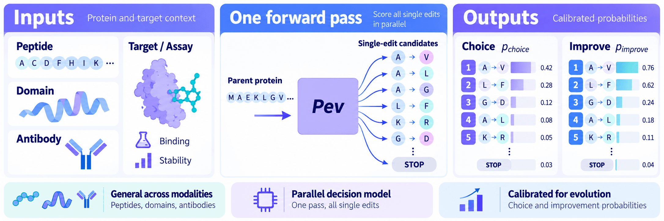
Pev is a general mutation policy for protein design. One set of weights, trained once on measured outcomes from many protein families, proposes edits for novel families, across peptides, small folded domains, and antibodies, under either binding or stability. It turns one parent encoding into parallel probabilities over all possible single substitution and STOP.

One pass per decision. A decision costs one forward pass, not one per candidate. At 1,000 candidates in a single request that is over 800× the throughput of an identical per-mutant encoder.
Zero-shot on novel families. A family-specific model needs measurements on that family, so a general policy is available exactly when assays are scarcest.
Calibrated probabilities. Beyond just a bare ranking, both heads are trained with proper scoring rules and calibrated post-hoc on held-out families.

This project is inspired by TypeSafe’s Jev, the first model of this class. What that means, and what it does not, is spelled out below.

Jev for science: a System One model for protein design

Jev is TypeSafe’s first System One model: state in, typed probabilistic decisions out, every option scored in one parallel pass. A round of directed evolution already has that shape. Pev is what it looks like filled in.

What is a System One model?

The name follows Kahneman’s System 1, fast and structured, as against the deliberate reasoning of a chat model. Three properties define the class and Pev has all three: typed output rather than text to parse, here every allowed substitution plus STOP; parallel scoring in one forward pass, worth 800× over a per-mutant encoder; and calibrated probabilities rather than a bare ranking.

Is there a System One model for science?

Pev is one, for protein design. One set of weights screens peptides, folded domains, and antibodies it has never seen, with no per-target fitting, and returns a beneficial mutation in 2 of every 5 wells against random screening’s 1 in 7. The results below are the evidence.

How does Pev differ from Jev?

Jev is general-purpose and proprietary, trained with TypeSafe’s unpublished RLCD recipe. Pev is open and domain-specific: ESM-2 650M with LoRA, supervised on measured assay outcomes under proper scoring rules, calibrated on held-out families. The two share the interface, not the recipe.

Is Pev affiliated with TypeSafe, or built on Jev?

No. Pev is an independent academic project from Northwestern University, not a TypeSafe product and not a reproduction of Jev. Jev is where the framing comes from, and it is cited as such.

Decision model for protein evolution

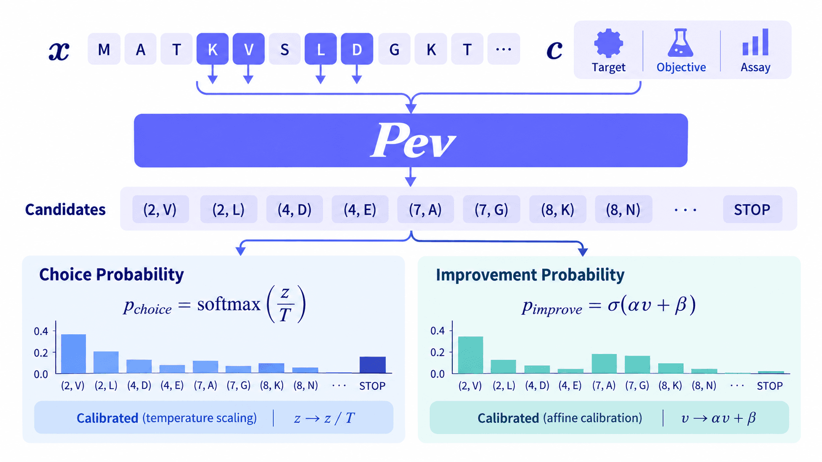
At each round the policy sees a parent sequence $x$ and an assay context $c$ , and returns either a single substitution $a = (i, r)$ , meaning residue $r$ at position $i$ , or STOP, meaning retain the best measured sequence. The model is history-free: it conditions on the current parent and context, not on a trajectory.

Pev method: parent sequence and assay context enter one encoder pass, which scores every allowed single substitution and STOP in parallel, emitting a temperature-calibrated choice distribution and an affine-calibrated improvement probability per edit. — **One pass, two calibrated answers.** The parent is encoded once and every allowed edit rides along on that single encoding. The sections below decompose this picture.

Architecture

ESM-2 650M with rank-16 LoRA on the query and value projections of the final four layers; everything below runs frozen. On top sit two-layer MLP heads, assay and readout embeddings, and projected target or partner context.

Parallel candidate scoring

This is the controlled comparison, and the reason a decision costs one backbone pass rather than one per candidate. The two arms differ in exactly one place:

Where candidate features come from
Model	Candidate representation
Pev parent_reuse	Reuse the parent encoding for every allowed edit
Per-mutant ESM+MLP per_mutant	Build $x \oplus a$ and encode each mutant separately

Heads, conditioning, losses, episodes, and candidate panels are identical. The only difference is where candidate features come from.

Two heads, two different events

The choice head is a softmax over the allowed edits together with STOP, so it sums to one. The improvement head is an independent sigmoid per edit, so these do not sum to one, because several edits can each be likely:

\begin{aligned} p_{\text{choice}}(a) &= \operatorname{softmax}\big(s_\theta(\cdot \mid x, c)\big)_a \quad \text{over } \mathcal{A}(x) \cup \{\mathrm{STOP}\} \\[4pt] p_{\text{improve}}(a) &= \sigma\big(v_\theta(a \mid x, c)\big) \;\approx\; \Pr\big[\,y(x \oplus a) > y(x)\,\big] \end{aligned}

One is not a substitute for the other. A best edit can carry a low improvement probability when every edit on offer is poor, which is precisely when STOP is the right call.

Training

\mathcal{L} \;=\; \mathbb{E}\big[\, \ell_{\text{choice}} + \lambda \cdot \ell_{\text{improve}} \,\big], \qquad \lambda = 1

Both terms are proper scoring rules. Losing candidates stay in the choice denominator, and nothing is class-weighted, oversampled, or label-smoothed, since each of those would move the probability target. Censored measurements are never treated as failures. Splits are by family, and a family held out for one property stays held out for every property.

Calibration

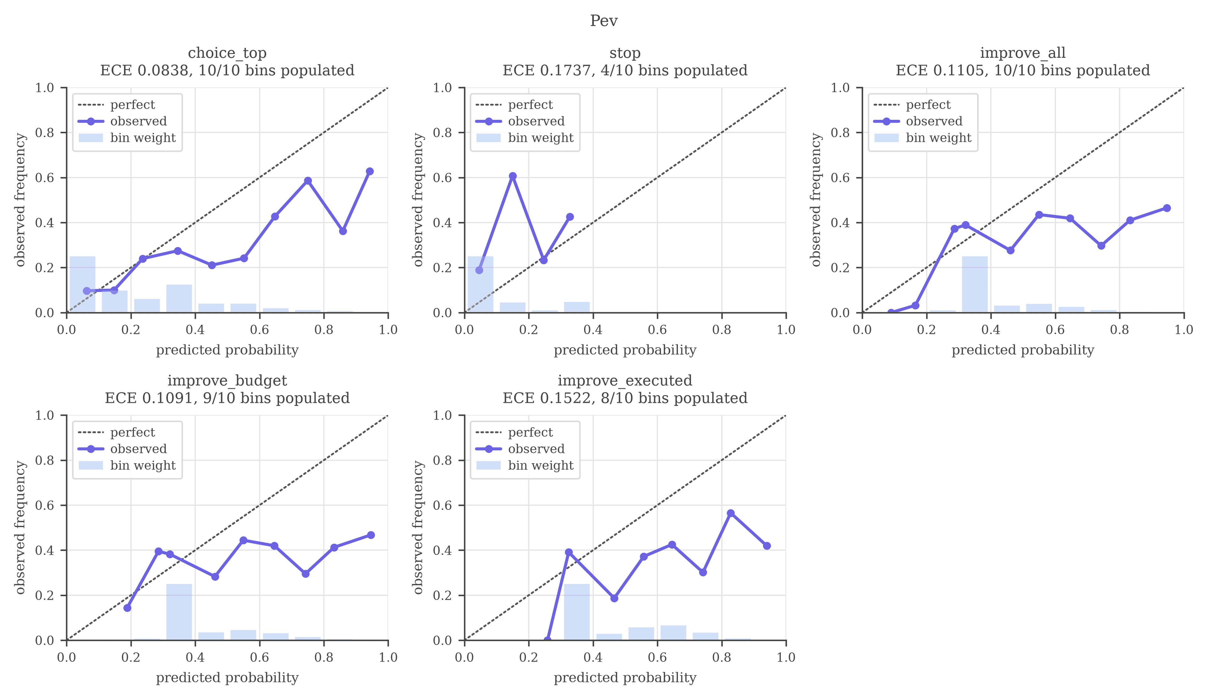
Raw scores rank edits well but are not yet probabilities. Two transforms fix that, one per objective: a temperature on the choice logits, and an affine shift on the improvement logit. Both are fitted on held-out calibration families, never on validation, whose logits are biased by checkpoint selection. Because both transforms preserve rank, they change what the model reports and never what it chooses: every decision metric is identical before and after.

Finding beneficial mutations in unseen families

The primary test. A panel is one measured reference protein and every measured single substitution of it, drawn from families reserved before training. A lab gets ten wells. Nothing is padded: an unmeasured mutation is absent from the panel, never counted as a miss. An edit counts as beneficial when it clears both replicate noise and a meaningful effect fixed in advance.

Discovery screen · ten wells, held-out families
Method	Hit rate @10 ↑	Enrichment @10 ↑	AUROC ↑	Wells to first hit ↓
Perfect ranking ceiling	0.951	19.4×	1.000	1.0
Pev one set of weights	0.410	6.82×	0.739	3.6
ESM-2 zero-shot untrained backbone	0.263	3.07×	0.546	51.0
Random floor	0.139	1.02×	0.497	29.2

Pev returns a beneficial mutation in 2 of every 5 wells where random screening returns 1 in 7. Paired family by family it clears both random and the untrained backbone, so this is what training buys rather than the pretrained prior, and it holds across seeds.

By sequence class · hit rate @10 ↑, with enrichment @10 beneath
Class	Pev	ESM-2 zero-shot	Random
Domain 27 families · 27 panels	0.4449.22×	0.2193.74×	0.0801.05×
Peptide 7 families · 13 panels	0.3001.44×	0.2791.27×	0.2300.99×
Antibody 5 families · 5 panels	0.3801.40×	0.4802.03×	0.3310.95×

Domain carries the result. Nine-fold enrichment and 0.823 AUROC against a random floor of 1.05×.
Peptide improves the ordering but not the yield. It clears random on ranking and barely on hit rate.
Antibody is unresolved on five families, and there the untrained backbone ranks better.

Binding lags for want of data, not tuning. A scan panel needs a measured reference plus its measured substitutions. Stability data is already that shape and most of it survives the requirement; binding data is not, and almost none of it does. No recipe among the twelve tried fixed that, including one built specifically to. What would is scan-shaped binding data: deep mutational scans of antibody–antigen pairs and receptor-binding domains.

Transfer to sparse measured neighbourhoods

A secondary diagnostic on the panels the corpus supplies everywhere else: a measured parent and its measured single-edit neighbours, a median of sixteen, half of which already improve it. A ten-well budget exceeds the number of hits on most of them, so the screening metrics saturate and only the two budget-free numbers are worth reading. Success@1 counts an episode correct when the chosen edit improved the parent or when the model correctly declined to spend the assay; it is the one place STOP is scored.

Sparse neighbourhoods · held-out families
Method	Success@1 ↑	Panel AUROC ↑
Perfect decisions ceiling	1.000	1.000
Pev neighbourhood-trained	0.502	0.575
Per-mutant main baseline	0.475	0.549
Choice-only no improvement loss	0.437	0.570
ESM-2 zero-shot untrained backbone	0.425	0.549
Pev scan-trained, reported above	0.402	0.542
Random floor	0.386	0.517
Regression no decision objective	0.357	0.563

The two panel shapes trade against each other. The scan-trained checkpoint that wins the discovery test does not clear random here; the neighbourhood-trained one does, and loses the discovery test. Training on both at once was worse at discovery than either specialist. The reported Pev is the discovery model, and this table records what that cost. Every method sits far closer to random than to perfect, so transfer to arbitrary neighbourhoods is largely unsolved either way.

Reliability diagrams after calibration, showing predicted probability against observed frequency for the choice and improvement heads. — **Reliability after calibration.** Predicted probability against observed frequency on held-out families. Points near the diagonal mean the reported numbers read as probabilities rather than as a bare ranking. The post-hoc fit improves every forecast here, though the model remains overconfident.

Better sequences per assay in a closed loop

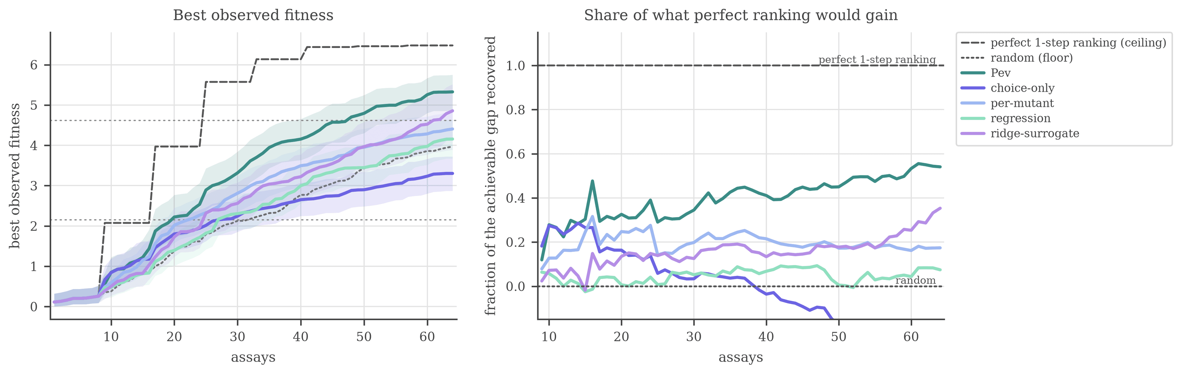
A closed-loop campaign on the GB1 four-site landscape, a target Pev has never seen. The comparison that matters is the ridge surrogate refit on the target’s own assays every round, which is what a practitioner actually reaches for.

GB1 four-site landscape · best observed fitness ↑
Assays	Random	Fitted surrogate	Per-mutant	Pev	Perfect ranking
16	0.85	1.03	1.12	1.44	2.08
32	2.17	2.74	2.90	3.61	5.57
64	3.97	4.86	4.53	5.33	6.48

Pev beats random at every budget and beats the fitted surrogate at the smaller ones, narrowing as the surrogate accumulates data. That narrowing is the point. The claim is that a general policy is useful before a target-specific one can be fitted, and the crossover is what makes it falsifiable.

Best observed fitness plotted against assay budget for Pev, a fitted ridge surrogate, the per-mutant, regression and choice-only variants, a random floor, and a perfect one-step ranker. — **Best observed fitness against assay budget.** The right panel rescales by what *perfect one-step ranking* would gain, not by the landscape maximum, so the remaining headroom is the limit of single-edit walks rather than of the model. The budget stops at 64 because past that, coverage substitutes for ranking.

Pareto frontier with one-pass scoring

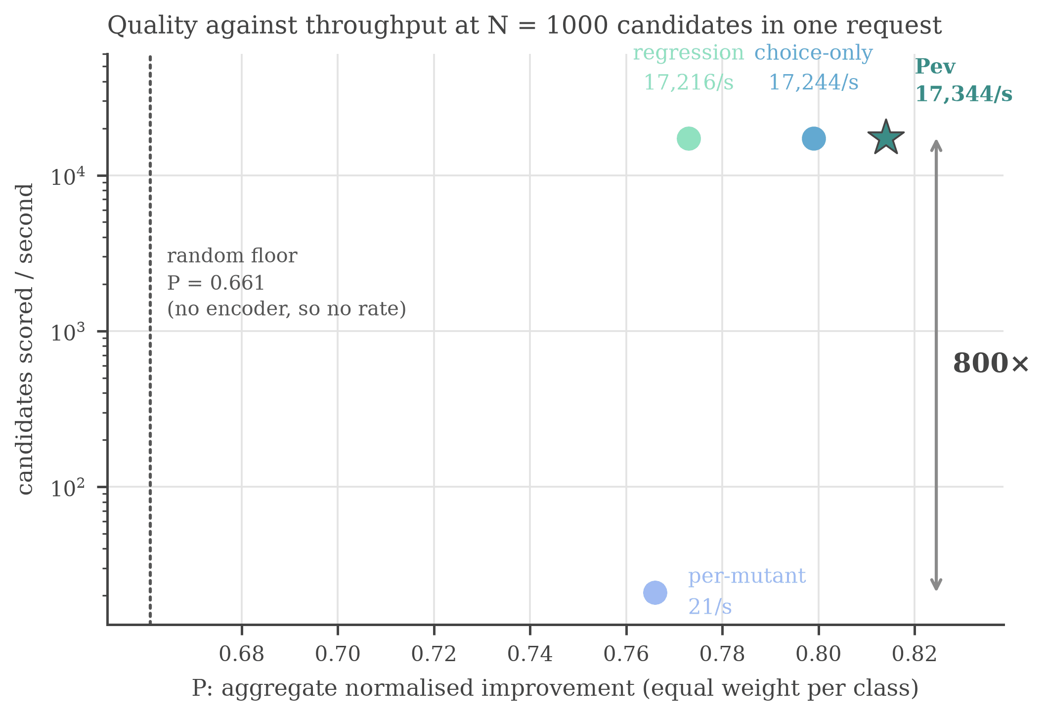
Scoring candidates in parallel is not a trade of accuracy for throughput. Against the per-mutant baseline it is a Pareto improvement: orders of magnitude more candidates per second, at quality within noise of it. Four variants trained identically on the current corpus isolate what parent reuse costs and buys.

Quality vs. throughput at $N = 1000$ candidates
Method	Improvement $P$ ↑	Candidates/s ↑
Pev parent reuse	0.814	17,344
Choice-only no improvement loss	0.799	17,244
Regression no decision objective	0.773	17,216
Per-mutant ESM+MLP main baseline	0.766	21
Random floor	0.661	n/a

Parent reuse keeps request latency roughly flat as the candidate count grows, while the per-mutant encoder pays for every candidate it scores, so the gap widens with request size: over 800× the throughput at $N = 1000$ , and here at the best quality of any variant. Pev is the only point on the frontier.

Candidates scored per second plotted against aggregate normalised improvement at 1000 candidates in one request, with Pev starred at the top right and the per-mutant baseline three orders of magnitude below it. — **Quality against throughput.** The per-mutant baseline sits three orders of magnitude below at comparable quality. Random has no encoder, so it is drawn as a quality floor rather than a rate.

What the results show

One policy, no per-target fitting. One set of weights screens peptides, folded domains, and antibodies it has never seen, under either binding or stability.
Three times the hit rate of random screening. Ten wells return a beneficial mutation in 2 of every 5 against random’s 1 in 7, at 6.82× enrichment and 9.22× on folded domains.
It beats the model a practitioner would fit. In closed loop on GB1 it outruns a ridge surrogate refit on that target’s own assays, where assays are scarcest.
800× the throughput at no quality cost. Parent reuse is a Pareto improvement over an identical per-mutant encoder, at the best quality of any variant measured.

Folded domains carry the deepest evidence, and binding is waiting on scan-shaped data rather than on further tuning.

BibTeX

@misc{wen2026pev,
  title={A System One Approach to General Protein Evolution},
  author={{Pev Team}},
  year={2026},
  eprint={XXXX.XXXXX},
  archivePrefix={arXiv},
  url={https://arxiv.org/abs/XXXX.XXXXX},
}